Parametric Density Estimation: Gaussian Distribution

가우시안 분포는 continuous random variable의 분포를 나타낼 때 사용한다.

보통 mean과 variance 두 parameter에 의해서 통제된다는 특징이 있다.

가우시안 분포는 다음과 같이 나타낼 수 있다. 이 때 x는 random variable이고, μ와 σ는 parameter이다.

 

Mean과 covariance를 사용하거나, information vector와 information matrix를 사용하면 다음과 같이 나타낼 수 있다. 

Information vector와 matrix를 사용한 형태를 dual form이라고 한다.

 

 

Distance for Gaussian

가우시안 분포를 mean vector와 variance matrix를 사용하면 다음과 같이 나타낼 수 있다.

이 때 가우시안 분포에 대해 거리를 구하는 방법으로는 Mahalanobis distance를 사용한다.

 

Variance matrix인 시그마는 diagonal matrix이므로 inverse는 성분들의 역수로 이루어진 diagonal matrix이다.

헷갈리면 https://www.cuemath.com/algebra/inverse-of-diagonal-matrix/를 참조하자.

만약 x가 scalar여서 variance가 identity matrix이면 위의 Mahalanobis distance가 Euclidean distance와 같아짐을 안다.

위의 정의로부터 변수에 대한 분산이 커지면 Mahalanobis distance는 작아짐을 알 수 있다.

이는 물체 인지에서 활용할 수 있는데, A와 B의 위치를 추정한다고 생각해보자.

A와 B의 Euclidean distance가 동일할 때, A의 분산이 B의 분산보다 작다고 가정하자.

그럼 B의 Mahalanobis distance는 A보다 작아진다.

이것은 불확실성을 고려할 때, B를 A보다 가깝게 인식할 수 있다는 것을 의미한다.

 

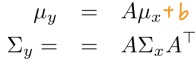
Gaussian and Systems

당연하게도 input이 가우시안 분포를 따르면, output도 가우시안 분포를 따른다.

Input-output 관계가 아래와 같을 때, output의 평균과 분산은 다음과 같이 나타낼 수 있다.

 

Conditional / Marginal distribution

이는 변수가 여러개 일 때, 쪼개서 분포를 나타낼 때 사용하는 방법으로 보인다.

변수를 임의로 나누어 평균과 분산을 다음과 나타낸다고 하자.

그럼 Conditional Guassian distribution은 p(a|b)로 나타낼 수 있고, Marginal Gaussian distribution은 p(a)로 나타낸다.

이 때 각각의 분포는 다음과 같은 Gaussian distribution을 따르고, 각각의 평균과 분산은 아래에 나타내두었다.

 

MLE / MAP for Gaussian

MLE와 MAP를 이용해서 평균을 추정하면 다음과 같이 나타낼 수 있다.

 

Covariance를 MAP를 이용하여 추정해보자.

이 때 precision이라는 새로운 parameter를 도입하여 다음과 같은 형태로 나타낼 수 있다.

이 형태는 Gamma function과 같은 형태이므로 감마 함수를 prior로 사용할 수 있다.

Prior인 감마 함수와 likelihood를 곱하여 다음과 같이 나타낼 수 있다.

 

Multivariate Gaussian precision matrix에 대해서는 prior를 Wishart distribution을 사용한다고 한다.

이는 이후 필요하면 추가적으로 공부하자.

 

 

Stuents's t-Distribution

Gaussian와 Gamma prior를 가정하면 다음과 같이 marginal distribution을 나타낼 수 있다.

사실 다 이해한 건 아니라서 이것도 필요하면 나중에 추가적으로 공부하자.

 

 

from elice_utils import EliceUtils

from sklearn.mixture import GaussianMixture

import cv2

import numpy as np

import matplotlib.pyplot as plt

elice_utils = EliceUtils()

def plt_show():

    plt.savefig("fig")

    elice_utils.send_image("fig.png")

def GMM_segmentation(image, classes):

    # Reshape image array to be (h, w, c) -> (h*w, c)

    h, w, c = image.shape

    image_array = image.reshape(-1, c)

   

    # TODO: Create a Gaussian Mixture Model with 'full' covariance type

    gmm = GaussianMixture(n_components=classes, covariance_type='full', random_state=42)

   

    # TODO: Fit the GMM to the RGB data

    'image_array 객체를 gmm 이용해서 훈련시키겠다는 의미'

    gmm.fit(image_array)

   

    # Predict clusters for each pixel

    'GMM 이용해서 분포된 cluters의 label을 예측해서 labels 객체에 저장'

    labels = gmm.predict(image_array)

   

    # Replace each pixel value with its cluster's mean RGB value

    segmented_image_array = np.zeros_like(image_array)

    for cluster_id in range(classes):

        # Retrieve the mean color

        mean_color = gmm.means_[cluster_id]

        # Match whether it belongs to the same cluster with the segmentation results

        'labels랑 cluter_id가 같은 것은 mean_color로 변환시켜 버림'

        segmented_image_array[labels == cluster_id] = mean_color

    # Reshape back to the original image shape

    '원래는 픽셀값만 가지고 있었는데, 이거를 다시 hwc 형태로 변환'

    segmented_image = segmented_image_array.reshape((h, w, c))

    return segmented_image

def main():

    image_path = './shrek.jpg'

    image = cv2.imread(image_path)

    image = cv2.cvtColor(image, cv2.COLOR_BGR2RGB)

   

    # Choose the number of Gaussian components

    classes = 10  # You can change this to any desired number

   

    segmentation = GMM_segmentation(image, classes)

    # For Visualizations

    plt.subplot(1, 2, 1)  # 1 row, 2 columns, 1st subplot

    plt.imshow(image)

    plt.title('Original Image')

    plt.axis('off')

    # Displaying the segmented image

    plt.subplot(1, 2, 2)  # 1 row, 2 columns, 2nd subplot

    plt.imshow(segmentation.astype(np.uint8))

    plt.title(f'Segmented Image (Gaussians={classes})')

    plt.axis('off')

    plt.tight_layout()

    plt_show()

if __name__ == "__main__":

    main()

 

from elice_utils import EliceUtils

import numpy as np

elice_utils = EliceUtils()

def euclidean_distances(x):

    """

    TODO: compute the Euclidean distance observed from person A and person B

   

    """

   

    distance_A = abs(x - 3)

    distance_B = abs(x - 2.7)

    return [distance_A, distance_B]

def mahalanobis_distances(x):

    """

    TODO: compute the Mahalnobis distance observed from person A and person B

   

    """

    distance_A = np.sqrt((x - 3) * 25 * (x - 3))

   

    distance_B = np.sqrt((x - 2.7) * 100 * (x - 2.7))

   

    return [distance_A, distance_B]

   

def estimate_error(person1, person2):

   

    mu_A, sigma_A = person1

    mu_B, sigma_B = person2

    mu_f = (mu_A * (sigma_B ** 2) + mu_B * (sigma_A ** 2)) / (sigma_A ** 2 + sigma_B ** 2)

    return mu_f

def main():

    person1 = [3, 0.2]

    person2 = [2.7, 0.1]

    x = 5

if __name__ == "__main__":

    main()

from elice_utils import EliceUtils

import numpy as np

elice_utils = EliceUtils()

def main():

   

    A = np.array([[3, 10], [-2,7]])

    b = np.array([-4, 3])

   

    x_mu = np.array([1, -2])

    x_cov = np.array([[10, -2], [-2, 4]])

   

    # TEST your compute_mean and compute_covar function before you submit!

                   

    #elice_utils.send_image('elice.png')

    #elice_utils.send_file('data/input.txt')

def compute_mean(A,b,mu):

    """

    TODO: compute the new mean

   

    Return:

   

    new_mean: {dtype=numpy.array}

   

    Computed new mean

   

   

    """

    new_mean = np.dot(A, mu) + b

    return new_mean

def compute_covar(A, covar):

    """

    TODO: compute the new covariance

   

    Return:

   

    new_cov: {dtype=numpy.array}

   

    Computed new covariance

   

   

    """

    new_cov = A @ covar @ A.T

    return new_cov

if __name__ == "__main__":

    main()